Paving the Way Towards Low-Overhead Uncertainty Calibration

An Accessible Intro to Laplace Approximations in Julia for Bayesian Deep Learning

A guest blog post by a team of students from TU Delft, who have contributed multiple improvements to LaplaceRedux.jl.

Guest Blog Post

This blog post was originally written by Severin Bratus and colleagues from TU Delft and published on Medium. This version of the post includes only minor edits. If you would like to contribute a guest blog post, please get in touch.

This post summarizes a quarter-long second-year BSc coursework project at TU Delft. Our team of five students has made multiple improvements to LaplaceRedux.jl, due to Patrick Altmeyer. Inspired by its Pythonic counterpart, laplacet-torch, this Julia library aims to provide low-overhead Bayesian uncertainty calibration to deep neural networks via Laplace Approximations (Daxberger et al. 2021).

A nice image to attract your attention. The exact inverse Fisher information matrix for a MNIST classifier network (left), its block-diagonal and tri-block-diagonal approximations (middle), and the absolute error (right). Source: Martens & Grosse (2015)

We will begin by demystifying the technical terms in the last sentence, in order to explain our contributions to the library and highlight some impressions from the experience. Note that our team has begun working on this PhD-tier subject only having had some introductory courses on probability and statistics, machine learning, and computational intelligence, without any prior exposure to Julia.

Bayesian Learning

Uncertainty calibration remains a crucial issue in safety-critical applications of modern AI, as, for instance, in autonomous driving. You would want your car autopilot not only to make accurate predictions but also to indicate when a model prediction is uncertain, to give control back to the human driver.

A model is well-calibrated if the confidence of a prediction matches its true error rate. Note that you can have well-fit models that are badly calibrated, and vice versa (just like in life, you meet smart people, yet annoyingly arrogant).

The standard deep learning training process of gradient descent converges at a weight configuration that minimizes the loss function. The model obtained may be great, yet it is only a point estimate of what the weight parameters should look like.

However, with the sheer immensity of the weight space, neural networks are probably underspecified by the data (or, overfit). As neural networks can approximate highly complex functions, many weight configurations would yield roughly the same training loss, yet with varying abilities to generalize outside the training dataset. This is why there are so many regularization methods out there, to keep the models simpler. One radical, yet effective approach is described by LeCun, Denker, and Solla (1989):

… it is possible to take a perfectly reasonable network, delete half (or more) of the weights and wind up with a network that works just as well, or better.

Figure 1: The loss landscape. One can imagine gradient descent as a particle, let’s say a ball, or a grain of sand, rolling to the bottom of a pit. Then for Bayesian Learning, we have as if a pile of sand poured around at that bottom point, with the pile being thicker where loss is lower. This proverbial sand pile would represent the posterior parameter distribution. Figure due to Amini et al. (2019)

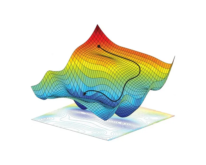
The way gradient is usually illustrated is with a picture like the one shown in Figure 1 above a curved terrain of the loss function across the parameter space. Each point of the horizontal plane corresponds to some configuration of parameters. Gradient descent seeks the point at the bottom of this terrain, as the point with the lowest loss, however as the loss-curvature is highly non-convex and high-dimensional there are many directions in which we could move and still maintain a low loss. Thus instead of a singular point we would like to specify a probability distribution around that optimal point. Bayesian methods, and in particular Laplace Approximations, allow us to do this!

Firstly, the Bayesian approach to neural network uncertainty calibration is that of modelling the posterior using Bayes’ Theorem:

\[ p(\theta \mid \mathcal{D}) = \tfrac{1}{Z} \,p(\mathcal{D} \mid \theta) \, p(\theta), \qquad Z:= p(\mathcal{D}) = \textstyle\int p(\mathcal{D} \mid \theta) \, p(\theta) \,d\theta \]

Here \(p(\mathcal{D} \mid \theta)\) is the likelihood of the data given by the parameters \(\theta\). The prior distribution \(p(\theta)\) specifies our beliefs about what the model parameters would be prior to observing the data. Finally, the intractable constant \(Z\) is called the evidence: it characterizes the probability of observing \(\mathcal{D}\) as a whole, across all possible parameter settings (see here for details).

For models returning a probability distribution (e.g. classifiers), the loss is commonly defined as the negative log-likelihood. Thus if gradient descent minimizes loss, it maximizes the likelihood, producing the maximum likelihood estimate (MLE), which (assuming a uniform prior) also maximizes the posterior. This is why we call this point the maximum a posteriori, or the MAP. It makes sense to model this point as the mode of the posterior distribution, which could, for example, be a normal Gaussian distribution (see also the introductory post on this blog).

Laplace Approximations

We do this by a simple-yet-smart trick introduced back in the late 18th century by Pierre-Simon Laplace, the self-proclaimed “greatest French mathematician of his time”. In general, the Laplace Approximation (LA) aims to find a Gaussian approximation to a probability density (in our case, the posterior) defined over a set of continuous variables (in our case, the weights) (Bishop 2006). We can then estimate the loss (negative log-likelihood) as its second-order Taylor expansion:

\[ \mathcal{L}(\mathcal{D}; \theta) \approx \mathcal{L}(\mathcal{D}; \theta_\text{MAP}) + \tfrac{1}{2} (\theta - \theta_\text{MAP})^\intercal \left( \nabla^2 _\theta \mathcal{L}(\mathcal{D}; \theta) \vert_{\theta_\text{MAP}} \right)(\theta - \theta_\text{MAP}) \]

Note that the first-order Taylor term vanishes at the MAP since it contains the gradient, and the gradient is zero at MAP, since MAP is a maximum, by definition. What remains is the constant (zeroth-order) term, and the second-order term, containing the Hessian, which is a matrix of partial second-order derivatives.

Then from this approximation, we can derive the long-sought multivariate normal distribution with the MAP as the mean, and the inverted Hessian as the covariance:

\[ p(\theta \mid \mathcal{D}) \approx N(\theta; \theta_\text{MAP}, \varSigma) \qquad\text{with}\qquad \varSigma := \left( \nabla^2_\theta \mathcal{L}(\mathcal{D};\theta) \vert_{\theta_\text{MAP}} \right)^{-1} \]

The evidence \(Z\) is now also tractably approximated in closed form, allowing us to apply the Bayes’ theorem, to obtain the posterior distribution \(p(\theta \mid \mathcal{D})\). We can then express the posterior predictive distribution, for an input \(x_*\), prediction \(f(x_*)\), to obtain the probability for an output \(y\).

The evidence \(Z\) is now also tractably approximated in closed form, allowing us to apply the Bayes’ theorem, to obtain the posterior distribution \(p(\theta \mid \mathcal{D})\). We can then express the posterior predictive distribution, to obtain the probability for an output \(y\), given a prediction \(f(x_*)\) for an input \(x_*\).

\[ p(y \mid f(x_*), \mathcal{D}) = \int p(y \mid f_\theta(x_*)) \, p(\theta \mid \mathcal{D}) \,d\theta \]

This is what we are really after, after all — instead of giving one singular point-estimate prediction \(\widehat{y} = f(x_*)\), we make the neural network give a distribution over \(y\).

However, since the Hessian, a square matrix, defines the covariance between all model parameters (upon inversion), of which there may be millions or billions, the computation and storage of the Hessian (not to speak of inversion!) become intractable, as its size scales quadratically with the number of parameters involved. Thus to apply Laplace approximations to large models, we must make some simplifications — which brings us to…

Hessian approximations

Multiple techniques to approximate the Hessian have arisen from a field adjacent, yet distinct from Bayesian learning — that of second-order optimization, where Hessians are used to accelerate gradient descent convergence.

One such approximation is the Fisher information matrix, or simply the Fisher:

\[ F := \textstyle\sum_{n=1}^N \mathbb{E}_{\widehat{y} \sim p(y \mid f_\theta(x_n))} \left[ gg^\intercal \right] \quad\text{with}\quad g = \nabla_\theta \log p(\widehat{y} \mid f_\theta(x_n)) \large\vert_{\theta_\text{MAP}} \]

Note that if instead of sampling the prediction \(\widehat{y} ~ p(y \mid f(x_n))\) from the model-defined distribution, we take the actual training-set label \(y_n\), the resulting matrix is called the empirical Fisher, which is distinct from the Fisher, yet aligns with it under some conditions, and does not generally capture second-order information. See Kunstner et al. (2019) for an excellent discussion on the distinction.

Instead of the Fisher, one can use the Generalized Gauss-Newton (GGN):

\[ G := \textstyle\sum_{n=1}^N J(x_n) \left( \nabla^2_{f} \log p(y_n \mid f) \Large\vert_{f=f_{\theta_\text{map}}(x_n)} \right) J(x_n)^\intercal \text{with}\qquad J(x_n) := \nabla_\theta f_\theta(x_n) \vert_{\theta_\text{map}} \]

Here \(J(x_n)\) represents the Jacobian of the model output w.r.t. the parameters. The middle factor \(\nabla^2 …\) is a Hessian of log-likelihood of \(y_n\) w.r.t. model output. Note that the model does not necessarily output ready target probabilities — for instance, classifiers output logits, values that define a probability distribution only after the application of the soft-max.

Unlike the Fisher, GGN does not require the network to define a probabilistic model on its output (Botev, Ritter, and Barber 2017). For models defining an exponential family distribution over the output, the two coincide (Kunstner, Balles, and Hennig 2020). This applies to classifiers since they define a categorical distribution over the output, but not to simple regression models.

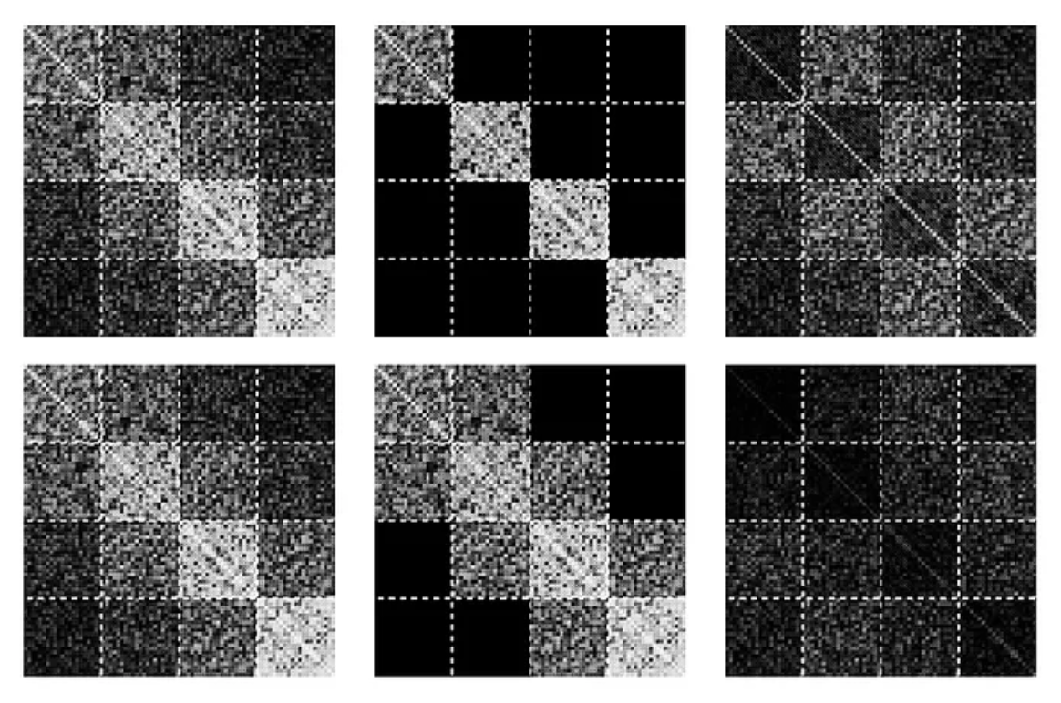
These matrices are quadratically large, it is infeasible to store them in full. The simplest estimation is to model the matrix as a diagonal — however one can easily contemplate how crude this approximation can be: for 100 parameters, only 1% of the full Hessian is captured.

A more sophisticated approach, due to Martens and Grosse (2015), is inspired by the observation that in practice the covariance matrices (i.e. inverted Hessians) for neural networks are block-diagonal-dominant. Thus we can effectively model the covariance matrix (and hence the Fisher) as a block-diagonal matrix, where blocks correspond to parameters grouped by layers. Additionally, each block is decomposed into two Kronecker factors, reducing the size of data stored several magnitudes more, at a cost of another assumption.

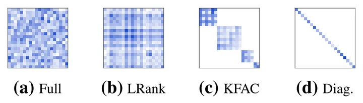
Lastly, a novel approach is to sketch a low-rank approximation of the Fisher (Sharma, Azizan, and Pavone 2021). Figure 2 shows four Hessian approximation structures:

Figure 2: (a) Hessian in full, intractable for large networks. (b) Low-rank. (c) Kronecker-factored Approximate Curvature, a block-diagonal method. (d) Diagonal. Source: Daxberger et al. (2021)

It is also possible to cut the costs by treating only a subset of the model parameters, i.e. a subnetwork, probabilistically, fixing the remaining parameters at their MAP-estimated values. One special case of subnetwork Laplace that was found to perform well in practice is last-layer Laplace, where the selected subnetwork contains only the weights and biases of the last layer.

Our contributions to LaplaceRedux.jl

In the scope of the project we have added support for: - multi-class classification, in addition to regression and binary classification; - GGN, in addition to empirical Fisher; - hardware-parallelized batched computation of both the empirical Fisher and the GGN; - subnetwork and last-layer Laplace; - KFAC for multi-class classification with Fisher; and - interfacing with MLJ, a common machine learning framework for Julia.

We have also made quality assurance / quality-of-life additions to the repository, adding: - a formatting check in the CI/CD pipeline; - an extensive test suite comparing the results of LaplaceRedux.jl against those of its Python counter-part package laplace-torch; and - a benchmark pipeline tracking possible downturns in performance.

Methodology

We adhered to the Agile/Scrum practices, with two-week-long sprints, and weekly meetings with our formal client, Patrick Altmeyer. We have prioritized the expected requirements by the Moscow method into must-, could-, should-, and won’t-haves. This is all fairly standard for BSc software projects at TU Delft. By the end of the project, we have completed all of our self-assigned must-haves and should-haves.

Pain Points

Here we list some obstacles we have encountered along the way: - Julia is slow to compile and load dependencies on less powerful machines. - Stack traces are sometimes rather obscure, though it seems to be the price to pay for macros. - Zygote.jl, the automatic differentiation library, is not self-autodifferentiable – it cannot differentiate its own functions. We would want this since we apply Zygote.jacobians when making predictions with the LA. - There is no accessible tool reporting branch coverage on tests – only line coverage is available. - Limited LSP and Unicode support for Jupyter Lab. - Conversion between Flux and ONNX is not yet implemented. - There is no extension library for Zygote equivalent to BackPACK or ASDL for second-order information.

• Zygote.jl, the automatic differentiation library, is not self-autodifferentiable: issue. We would want this since we apply Zygote.jacobians when making predictions with the LA.
• There is no accessible tool reporting branch coverage on tests – only line coverage is available.
• Limited LSP and Unicode support for Jupyter Lab.
• No conversion between Flux and ONNX is implemented yet ONNX.jl
• There is no extension library for Zygote equivalent to BackPACK or ASDL for second-order information.

Highlights

And here is what we found refreshing: - Metaprogramming and first-class support for macros are something completely different for students who are used to Java & Python. - The Julia standard API, and Flux/Zygote, are fairly straightforward to use, and well-thought-out for numerical computing and machine learning.

Conclusions

We have covered some elements of the theory behind Laplace Approximations, laid down our additions to the LaplaceRedux.jl package, and brought out some difficulties we, as complete newcomers to Julia, came across. Hope you have enjoyed the tour, and hopefully it has intrigued you enough to look deeper into Bayesian learning and/or Julia since both are developing at a lively pace. You can check out LaplaceRedux on the JuliaTrustworthyAI GitHub page here. Contributions and comments are welcome!

Acknowedgements

Our team members are Mark Ardman, Severin Bratus, Adelina Cazacu, Andrei Ionescu, and Ivan Makarov. We would like to thank Patrick Altmeyer for the opportunity to work on this unique project and for the continuous guidance throughout the development process. We are also grateful to Sebastijan Dumančić, our coach, Sven van der Voort, our TA mentor, and Antony Bartlett, our supporting advisor.

References

Amini, Alexander, Ava Soleimany, Sertac Karaman, and Daniela Rus. 2019. “Spatial Uncertainty Sampling for End-to-End Control.” arXiv. https://doi.org/10.48550/arXiv.1805.04829.

Bishop, Christopher M. 2006. Pattern Recognition and Machine Learning. springer.

Botev, Aleksandar, Hippolyt Ritter, and David Barber. 2017. “Practical Gauss-Newton Optimisation for Deep Learning.” arXiv. https://doi.org/10.48550/arXiv.1706.03662.

Daxberger, Erik, Agustinus Kristiadi, Alexander Immer, Runa Eschenhagen, Matthias Bauer, and Philipp Hennig. 2021. “Laplace Redux-Effortless Bayesian Deep Learning.” Advances in Neural Information Processing Systems 34.

Kunstner, Frederik, Lukas Balles, and Philipp Hennig. 2020. “Limitations of the Empirical Fisher Approximation for Natural Gradient Descent.” arXiv. https://doi.org/10.48550/arXiv.1905.12558.

LeCun, Yann, John Denker, and Sara Solla. 1989. “Optimal Brain Damage.” In Advances in Neural Information Processing Systems. Vol. 2. Morgan-Kaufmann. https://proceedings.neurips.cc/paper/1989/hash/6c9882bbac1c7093bd25041881277658-Abstract.html.

Sharma, Apoorva, Navid Azizan, and Marco Pavone. 2021. “Sketching Curvature for Efficient Out-of-Distribution Detection for Deep Neural Networks.” arXiv. https://doi.org/10.48550/arXiv.2102.12567.